Chapter 4 The normal distribution - what’s the point?
Many events can’t be predicted with total certainty. The best we can say is how likely they are to happen. Day to day, probability is often used to describe the world around. The chance of rain, the likelihood of our football team winning, or who will win the election. What do these statements actually mean and how are they calculated?
Hiding behind these statements is the idea of a probability distribution. This is a mathematical function that can be thought of as providing the probabilities of occurrence of different possible outcomes in an experiment. It is our way of trying to capture the real world using mathematics.
Probability is massive topic, that we cannot possibility hope to cover in a single chapter. Instead, the goal of this chapter is to give an intuitive feel for some of the standard probability distributions. Even if you have never taken a course in statistics, you’ll have come the simplest probability distribution already, the Uniform distribution. This distribution represents the situation where all events are equally likely
The most famous distribution is the Normal or Gaussian distribution. Instead of producing this distribution from thin air, we will provide some background to explain how this distribution naturally arises with few assumptions. In later chapters, the Normal distribution will form the basis for our inferential models.
Do I need to know this for data science? There are many people who no little about distributions, but “do data science”. In my opinion, having insight in the foundations will help you understand the subject, and hence allow you to build better models.
As an analogy, you can build web-pages using tools without knowing any HTML, CSS, or Javascript. However there comes a point where knowing the underlying technology is essential.
4.1 The Bernoulli distribution
The simplest distribution is the Bernoulli distribution. It models events that have only two outcomes. For example, your football team will either win or not. Since there are a countable number of events, this is a discrete distribution. This distribution forms the building block for all other distributions.
4.1.1 Motivating example
Suppose you are using a well know cloud provider. Reading the small print, they state that the chance of downtime on any particular day, is 0.001. What is the probability of having no downtime throughout the year?
4.1.2 Description
The easiest way to think of the Bernoulli distribution is to toss a (fair) coin. We have equally likely outcomes: heads and tails. Since they are equally likely, the probability6 of getting either event is 0.5. This means on average, 50% of throws will be heads and 50% of throws will be tails. The distribution that describes a coin throw is known as the Bernoulli distribution named after the Swiss scientist Jacob Bernoulli.
Mathematically we would describe the Bernoulli distribution as follows. Suppose \(X\) is a random variable7, then we have \[ \Pr(X = 0) = 1 - p \quad \text{and} \quad \Pr(X = 1) = p. \] Note that the total probability sums to \(1\), i.e. when we toss a coin, we will observe either a head or a tail.
If we simulated or observed a series of ten Bernoulli trials where \(p = 0.5\), this means we observe a series of \(0\)’s and \(1\)’s that follow the above probability distribution. It would look something like
0 0 1 0 0 1 0 1 0 0Notice that we don’t have exactly \(5\) ones. Instead, the probability distribution tells us that on average we’ll observe \(5\) ones.
Beware of the law of averages. Basically, just because you observe 3 heads in a row, the chance of observing a fourth head is still 0.5.
4.1.3 Example
Suppose you are using a data centre where the probability of failure is 0.001 per day. That means the probability of the data centre working is 0.999 per day. So the probability that the data centre will work two days in a row is \(0.999 \times 0.999 = 0.998\). The probability that it will work every day for a year is \[ 0.999 \times 0.999 \times \ldots = 0.999^{365} = 0.694. \]That means that even though we only expect one failure every one thousand days. The chance of a failure happening in the coming year is approximately 1 in 3, or \(1- 0.694 \simeq 0.3.\)
4.2 The Binomial distribution
4.2.1 Motivating example
You are in charge of back-ups. Looking at a recent study you estimate the chance of a particular hard drive failing within one year to be 5% (or 0.05). Your organisation has around 1,000 hard drives. You would like to know
- How many hard drives are likely to fail this year?
- Can we get a reasonable upper limit for the number of failures?
4.2.2 Description
The Binomial distribution is an extension to the Bernoulli distribution. The Binomial distribution concerns sums of Bernoulli random variables. So in our our above example we have \[ 0 + 0 + 1 + 0 + 0 + 1 + 0 + 1 + 0 + 0 = 3 \] The Binomial distribution has two parameters, \(n\) the number of trials and \(p\) the probability of success. The probability of getting exactly \(k\) successes in \(n\) trials is given by \[ \Pr(X = k) = \binom{n}{k} p^k (1-p)^{n-k} \] where \[ \binom {n}{k} = \frac {n!}{k!(n-k)!} \] and \(n! = n \times (n-1) \times (n-2) \times (n-3) \ldots\). Notice that when \(n = 1\), the Binomial distribution just becomes the Bernoulli distribution: \[ \Pr(X = 0) = \binom{1}{0} p^0 (1-p)^{1-0} = 1 \times 1 \times (1-p) = (1-p) . \] With a little bit of mathematics, we can show that if we performed \(n\) experiments, with each experiment having probability \(p\) of success, then the mean number of successful outcomes is \(n \times p\) and the variance is \(n \times p \times (1 - p)\).
4.2.3 What does the Binomial distribution look like?
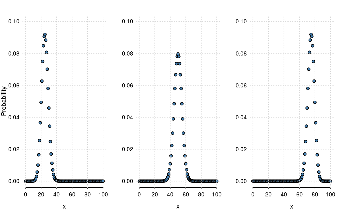
Let’s take a concrete example of \(n = 100\) and \(p = 0.25\), \(0.5\) and \(0.75\). The probability distributions are shown in figure 4.1.

Figure 4.1: The Binomial distribution with \(n=100\) and \(p =0.25\), \(0.5\) and \(0.75\).
Some points to note:
- The sum of points in each plot in figure 4.1 is \(1\). It’s a probability mass function, so it must sum to 1.
- The distribution is centred around the mean, \(n \times p\). So when \(p=0.5\), the plot is centred around \(50\).
- There is some variation around the mean. Again we can be more precise and state that the variance is \(n \times p \times (1-p)\). So when \(p = 0.5\), the variance is \(n/4 = 100/4 = 25\)
4.2.4 Motivating example
In our example we have \(n = 1000\) hard drives that fail with rate \(p = 0.05\). On average we would expect \(n \times p = 1000 \times 0.05 = 50\) failures per year. To obtain an upper bound, we would look at the cumulative distribution, that is,
\[ Pr(X \le k) = Pr(X = 0) + Pr(X = 1) + \ldots + Pr(X = k) \]
This is easily done in R. The function pbinom() calculates the probability of observing less than or equal to the value of it’s first argument. So to obtain a reasonable upper bound, we calculate the cumulative probability from \(0\) to \(1000\) and determine where it crosses the 0.99 probability threshold
n = 1000; p = 0.05
which(pbinom(0:n, n, p) > 0.99)[1]
#> [1] 68
Hence the probability that we observe more than \(67\) failures in one year is less that 0.01. So while the mean number of failures is 50, a reasonable upper bound would be 67.
4.3 The Normal/Gaussian distribution
A number of mathematicians contributed to the development of this distribution. The distributions namesake, Carl Friedrich Gauss was a German mathematician who developed a number of key statistical concepts, such as least squares optimisation.
The Normal distribution (or Gaussian) distribution is perhaps the most famous probability distribution. The previous distributions have been discrete, the Normal distribution is a continuous distribution. It takes the form \[ f_X(x) = \frac{1}{\sqrt{2 \pi \sigma^2}} e^{- \frac{(x - \mu)^2}{2 \sigma^2}} \] where
- \(\mu\) is the mean or expectation of the distribution (and also its median and mode);
- \(\sigma\) is the standard deviation;
- \(\sigma^2\) is the variance.
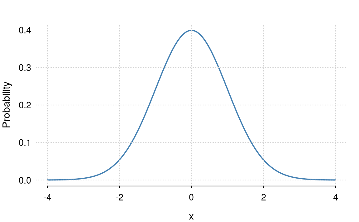
The standard normal distribution (figure 4.2) is a special case of the normal distribution where \(\mu = 0\) and \(\sigma = 1\) \[ f_X(x) = \frac{1}{\sqrt{2 \pi}} e^{- \frac{x^2}{2}} \]

Figure 4.2: The standard normal distribution: \(\mu=0\) and \(\sigma = 1\).
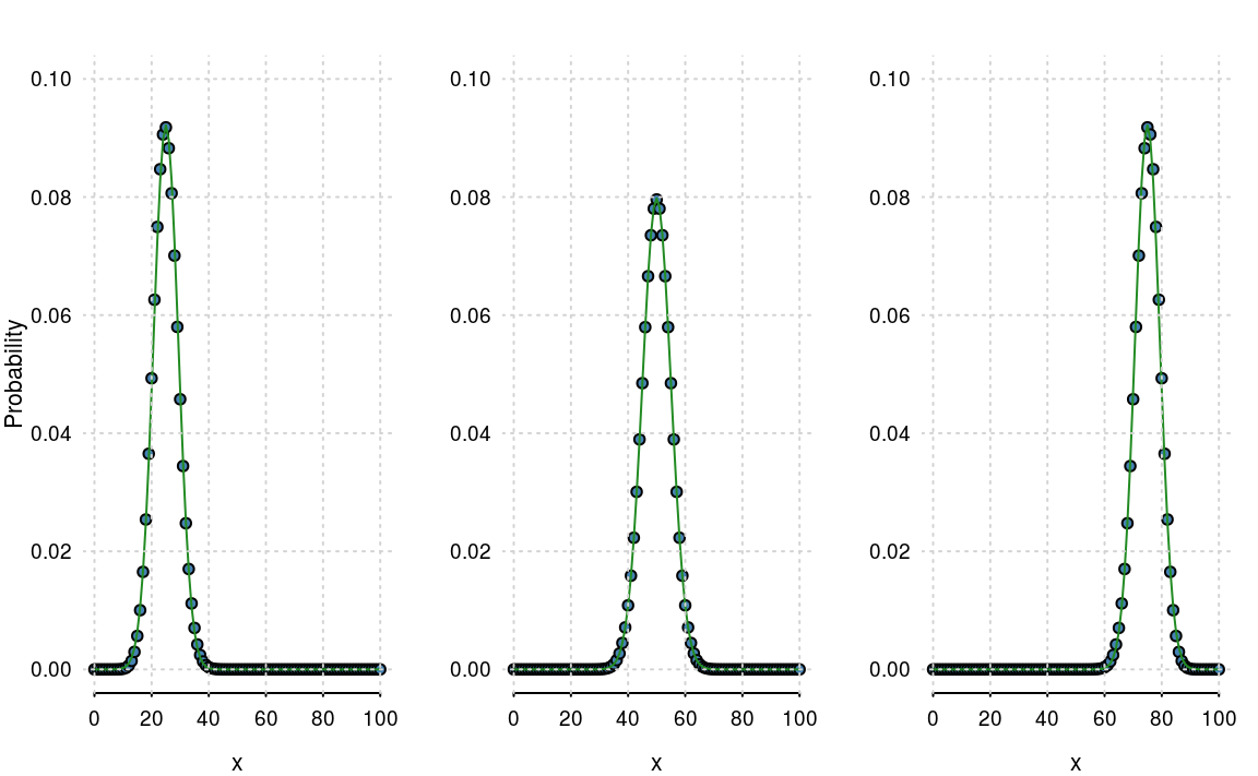
The distribution can be derived in a variety of ways, but the easiest is as a special case of the Binomial distribution. Letting \(n\) get large (basically when \(n > 20\)), and provided \(p\) isn’t too close to \(0\) or \(1\), the normal distribution is almost identical to the Binomial. Again, we can use mathematics to show that the binomial distribution converges to the normal, but to avoid unnecessary mathematical detail, we’ll just use a few plots (figure 4.3).

Figure 4.3: Binomial distributions with their normal approximations.
4.3.1 Continuous and discrete distributions
The Binomial and Bernoulli are examples of discrete distributions. A discrete distribution gives you the probability of observing a particular event such as rolling a dice or tossing a coin. For a discrete distribution, the probabilities will sum to \(1\), e.g. we will either get a head or tail, but one of the two events must happen.
A continuous distribution is a bit different. Looking at the formula for the normal distribution we see that it is valid for all values of \(x\). That means if we added up \(f_X(x)\) for all values of \(x\), we would reach \(\infty\), since \(x\) has infinitely many decimal places. Instead, for continuous distributions we look at area under the curve. So the area under the normal distribution sums (or integrates) to one.
4.3.2 The standard deviations rule
When your data are normally distribution, then the
- mean \(\pm\) 1 standard deviation: \(\simeq\) 70% of data;
- mean \(\pm\) 2 standard deviation: \(\simeq\) 95% of data;
- mean \(\pm\) 3 standard deviation: \(\simeq\) 99.9% of data.
This is way the mean and variance are useful summary statistics.
4.3.3 The Z-Score
The \(z\)-score is where we transform, or scale, the dataset to have mean \(0\) and variance \(1\). If our original data is \(x\), then our transformed data \(z\) is defined as \[ z = \frac{x - \bar x}{s} \] where \(\bar x\) is the mean of \(x\) and \(s\) is the standard deviation. The transformed data tells us how many standard deviations above or below the mean each data point is. If our data is normal, this would produce a standard normal distribution.
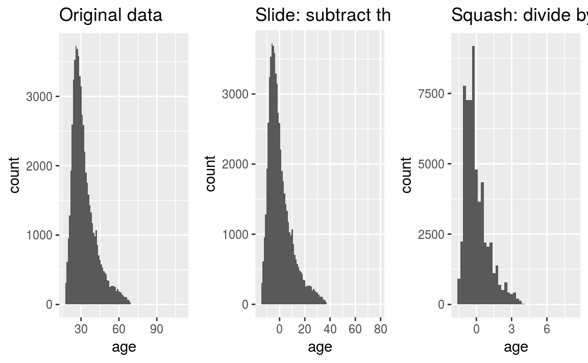
This is also known as “slide and squash rule”. Looking at the OKCupid data set again. The original distribution of ages is shown in figure 4.4 a.
- Subtract the mean, slides the distribution to \(0\) - figure 4.4 b.
- Dividing by the standard deviation, squashes the distribution to have a variance of \(1\) - figure 4.4 c.
Using \(Z\)-scores is a standard technique to put different variables on the same scale. This also helps many machine learning algorithms converge quicker.

Figure 4.4: The slide and squash rule.