Chapter 6 Capturing relationships with linear regression

In many data science problems, we wish to use information about some variables to help predict the outcome of another variable. For example, in banking, we might wish to use a persons financial history to predict the likelihood of them defaulting on a mortgage. The idea of using past data to predict future events is central to data science and statistics.

The simplest relationship between two variables is linear. The correlation coefficient will provide a single number summary of this relationship. To use the linear interaction for prediction, we need to use linear regression techniques. In our final chapter, we will look at standard modelling techniques.
We’ll start with the simplest measure, correlation, before moving onto linear regression models.

6.1 Capturing linear relationships

The easiest way to quantify the relationship between two variables is to calculate the correlation coefficient. This is a measure of the linear association. The sample correlation coefficient is defined as \[ r=\frac {\sum _{i=1}^{n}(x_{i}-{\bar {x}})(y_{i}-{\bar {y}})}{{\sqrt {\sum _{i=1}^{n}(x_{i}-{\bar {x}})^{2}}}{\sqrt {\sum _{i=1}^{n}(y_{i}-{\bar {y}})^{2}}}} \] where

\(n\) is the sample size;.
\(x_{i},y_{i}\) are the single samples indexed with \(i\).
\(\bar {x} = \frac {1}{n} \sum _{i=1}^{n} x_{i}\) is the (the sample mean).

The value of \(r\) lies between \(-1\) and \(1\). A value of \(1\) implies that all data points lie on a line as \(X\) and \(Y\) increase. A values of \(-1\) implies that all data points lie on a line where \(Y\) decreases as \(X\) increases. A value of 0 implies that there is no linear correlation between the variables.

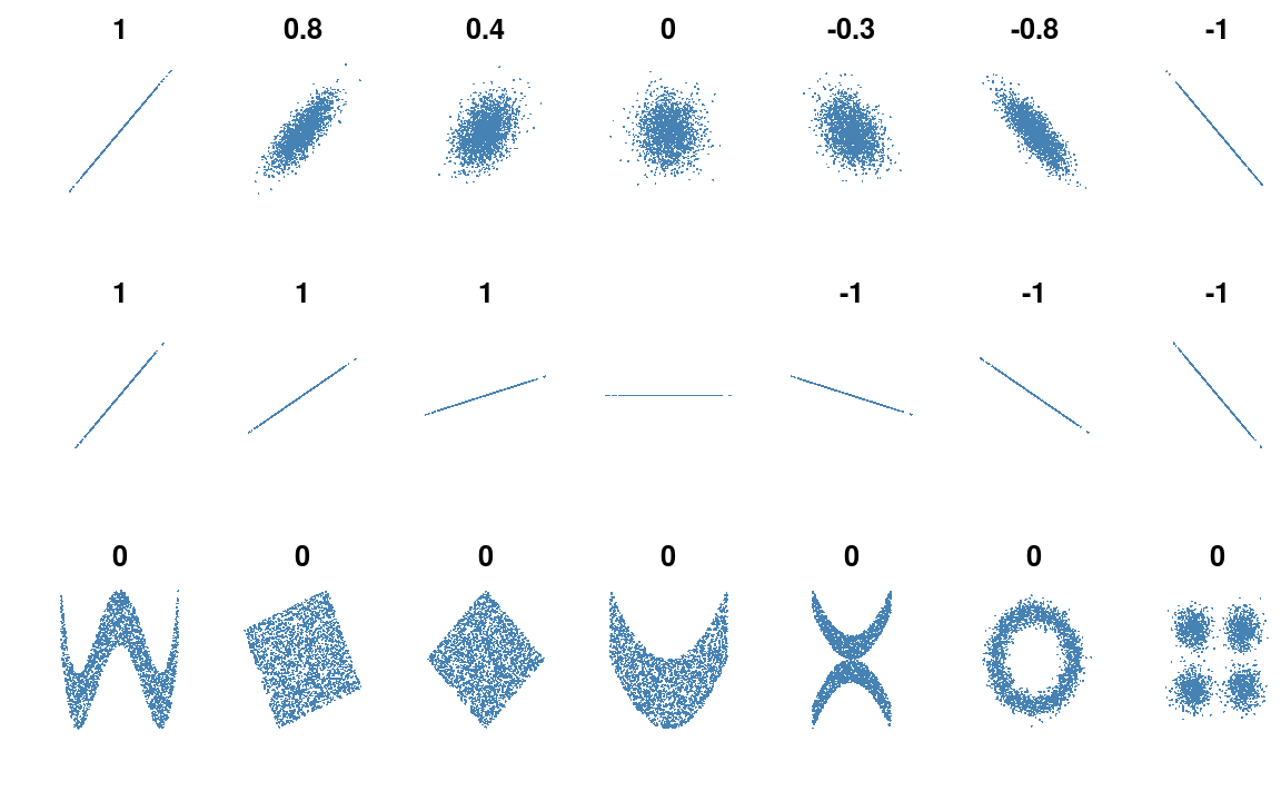
Figure 6.1: Several sets of (x, y) points, with the correlation coefficient of x and y for each set. Credit: Wikipedia

Figure 6.1 (shamelessly stolen from wikipedia) gives a very useful overview of the correlation coefficient. The top row of plot shows how data changes as we move from a coefficient of \(+1\) to \(-1\). When \(r = 0\), we just have random scatter.

Something that is often forgotten, is that correlation does not measure the strength of the linear association. This is clear from the second row of figure 6.1 where it is clear that the correlation does not depend on the gradient.

The final row of figure 6.1 shows figures where the correlation cofficient is 0. However, in each example there is clearly a relationship; it’s just not linear.

Calculating the correlation is a useful first step when you first come across a data set. My typical first step is to run image(cor(data_set)). This produces a very ugly, but informative heatmap of the correlation cofficients.

6.1.1 Example: Starbucks calorie content

The Starbucks data set contains nutritional value of 113 items. For each item on the menu we have the number of calories, and the carbohydrate, fat, fiber and protein amount.

We can quickly get an overview in R,

head(starbucks)
#>                                  Product Calories Fat Carb Fiber Protein
#> 1                           Chonga Bagel      300   5   50     3      12
#> 2                           8-Grain Roll      380   6   70     7      10
#> 3                       Almond Croissant      410  22   45     3      10
#> 4                          Apple Fritter      460  23   56     2       7
#> 5                       Banana Nut Bread      420  22   52     2       6
#> 6 Blueberry Muffin with Yogurt and Honey      380  16   53     1       6

and generate a few scatter plots 6.2.

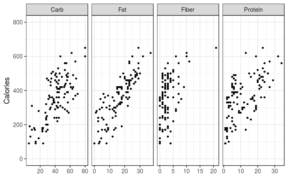
Figure 6.2: Relationships of Calories content and ingredients.

The scatter plots show a clear linear trend. To work out the sample pairwise correlations we use the cor() function

## Drop the first column since it's the food names
cor(starbucks[, -1])
#>          Calories   Fat  Carb Fiber Protein
#> Calories    1.000 0.829 0.708 0.471   0.619
#> Fat         0.829 1.000 0.281 0.276   0.423
#> Carb        0.708 0.281 1.000 0.408   0.204
#> Fiber       0.471 0.276 0.408 1.000   0.472
#> Protein     0.619 0.423 0.204 0.472   1.000

The R output returns all pairwise correlations between the 5 variables:

There is a diagonal of 1, since the correlation of a variable with itself is 1.
The matrix is symmetric since the correlation between \(X\) and \(Y\) is the same as the correlation between \(Y\) and \(X\).

Out of the four component parts, Fat is very highly correlated with Calories.

6.2 Linear Regression

The next step is use information about one variable to inform you about another. If you recall back to your school days, you’ll hopefully remember that the equation of a straight line is \[ Y = \beta_0 + \beta_1 x \] where

\(\beta_0\) is the \(y\)-intercept (in the UK, we used \(c\) instead of \(\beta_0\));
\(\beta_1\) is the gradient (in the UK, we used \(m\) instead of \(\beta_1\)).

In statistics, we usually call \(Y\) the response variable (the thing we want to predict) and \(x\) the predictor (or covariate). The aim of the model is to estimate the values of \(\beta_0\) and \(\beta_1\). However, since we only have a sample, there is uncertainity surrounding our estimate.

To fit the model in R, we use the lm()¹¹ function

# This is an R formula
# Read as: Calories is modeled by Fat
(m = lm(Calories ~ Fat, data = starbucks))
#> 
#> Call:
#> lm(formula = Calories ~ Fat, data = starbucks)
#> 
#> Coefficients:
#> (Intercept)          Fat  
#>       148.0         12.8

The output from R gives estimates of \(\beta_0 = 148.0\) and \(\beta_1 = 12.8\).

6.2.1 Prediction and Interpretation

The estimated model, \[ \text{Calories} = 148 + 12.8 \times \text{Fat} \] allows us to predict the calorie content based on the fat. For example, if the fat content was 10, then the estimated calorie content would be 276. However this simple example also highlights the potential dangers of using the model for prediction. If we wished to predict the calorie content of fat-free food, i.e. \(\text{Fat} = 0\), then our model would estimate the calorie content as \(148\). This seems a bit high for a glass of water! The obvious reason for this poor fit is that our model isn’t capturing our aspects of the relationship or is missing other significant covariates.

6.2.2 How do we estimate the model coefficients?

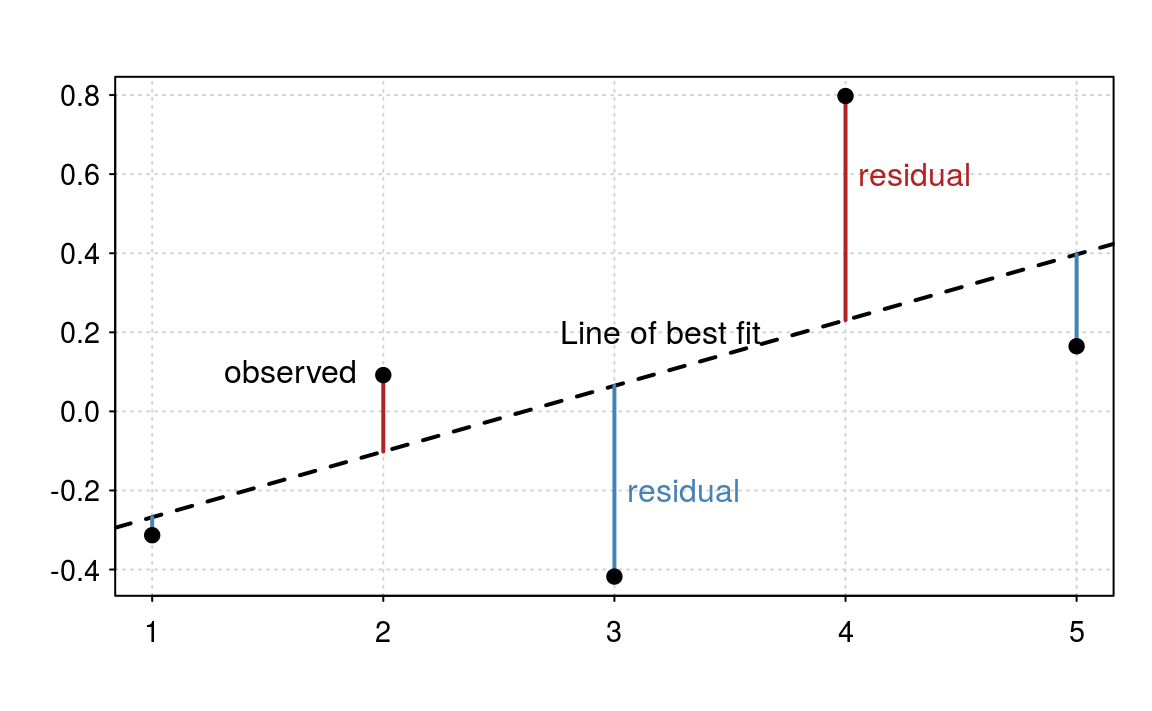
We estimate the model parameters by “minimising the sum of squared residuals”. A residual is the difference between the observed value and the predicted value. In figure 6.3, the observed values, i.e. the data, are the black dots and the residuals are the solid lines. The line of best fit is the dashed line. In figure 6.3 we have five data points, so we must have five residuals.

The classical statistics interpretation of a linear regression model is to assume the underlying model is actually \[ Y = \beta_0 + \beta_1 x + \epsilon \] where \(\epsilon\) is normally distributed. If assume that the errors (\(\epsilon\)) follow a normal distribution, then to estimate the parameter values we minimise the sum of squared residuals.

Figure 6.3: Residuals and linear regression.

The machine learning interpretation is that we have a cost function that we wish to minimise. It just so happens that in this particular case, that the cost function corresponds to assuming normality. But we could have used any cost function. To assess model fit, we would typically use Cross validation or a similar method.

One approach isn’t better than the other. The statistics approach gives more insight into the mechanisms, but the machine learning approach leads to a better predictive model. As in most cases, a combination of both methods is the optimal approach.

6.3 Multiple linear regression models

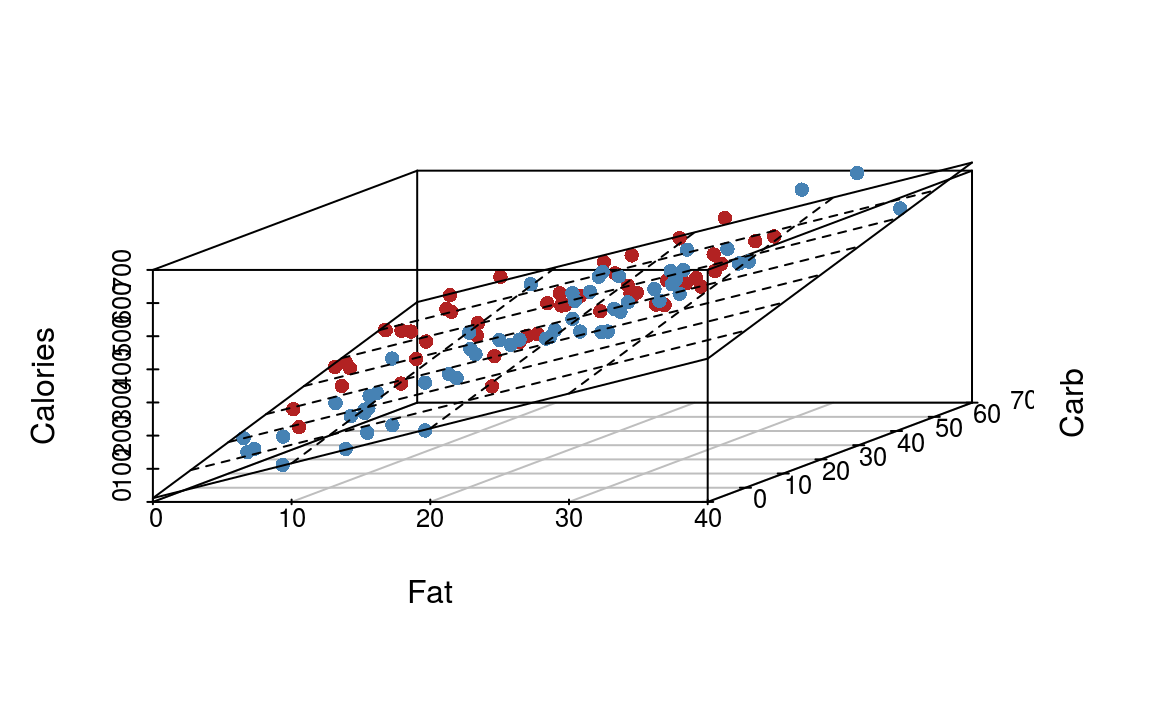
A multiple linear regression model is the natural extension of the simple linear regression model. If we have two predictors, e.g. \[ Y = \beta_0 + \beta_1 \text{Fat} + \beta_2 \text{Carb} \] This is equivalent to fitting a plane (a sheet of paper) through the points (figure 6.4).

Figure 6.4: Illustration of multiple linear regression with two predictor variables.

When we have more than two predictor variables, the geometric interpretation gets messy, but it’s still the same idea.

The parameter estimating procedure is identical to simple linear regression - we wish to minimise the sum of squared residuals. Furthermore, we still have the two views of the model: the statistical and machine learning.

Fitting the model in R is a simple extension

(m = lm(Calories ~ Fat + Carb, data = starbucks))
#> 
#> Call:
#> lm(formula = Calories ~ Fat + Carb, data = starbucks)
#> 
#> Coefficients:
#> (Intercept)          Fat         Carb  
#>       11.36        10.52         4.17

Notice that the coefficient for Fat has decreased from 12.8 to 10.52 due to the influence of the Carbohydrate component.

lm is short of linear model; this model is linear in the model coefficients.↩