Chapter 5 Margin of Error
Testing leads to failure, and failure leads to understanding Burt Rutan
5.1 Introduction & motativating example
Suppose we’re comparing two advert designs. At great expense, it has been decided to change the font to Comic Sans. Does this change work? Being a (data) scientist we decide to (humanely8) experiment on people by randomly showing them the advert. From past experience, you know that customers spent 45 seconds (on average) on your site. After switching to comic sans, we recorded the amount of time spent on the site by 20 customers
34 51 30 79 54 31 57 62 59 41 77 55 35 3 69 46 47 66 63 59Should we consider switching to comic sans?
Clearly time will vary visit–by–visit. On some visits, customers might spent more time (up to 79 seconds), but on others visits, they may only spend a few seconds. To get an overall impression, we could work out the average time for the above sample \[ \bar x = \frac{34 + 51 + 30 + \ldots + 59}{20} = 50.9 \] The new website does seem to be perform slightly better. But we have a very small sample. If we took another twenty visits, we would get a different estimate. We need to account for this sampling variability of the mean \(\bar x\), and the most common way of doing this is to perform a hypothesis test.
5.2 One sample test
The one–sample z–test can be useful when we are interested in how the mean of a set of sample observations compares to some target value. The mean in our sample, as always, is denoted by \(\bar x\). The standard notation in statistics for the population mean is the Greek symbol \(\mu\) (pronounced “mu”). Obviously, \(\bar x\) is our sample estimate of \(\mu\).
In the example above, we’d like to know whether our new font has affected the amount of time people spend on our site. In hypothesis testing, we make this assertion in the null hypothesis, denoted by \(H_0\) and often written down as \[ H_0: \mu = 45 \] We usually test against a general alternative hypothesis \(H_1\) \[ H_1: \mu \ne 45 \] which says “\(\mu\) is not equal to 45”.
When performing the hypothesis test, we assume \(H_0\) to be true. We then ask ourselves the question:
How likely is it that we would observe the data we have, or indeed anything more extreme than this, if the null hypothesis is true?
We can get a handle on this question thanks to the Central Limit Theorem in Statistics. Although we will not go into the details here, this result tells us that the quantity \[ Z = \frac{\bar x - \mu}{s/\sqrt{n}} \] follows a normal distribution (when \(n\) is reasonably large). In this formula
- \(\bar x\) is our sample mean;
- \(\mu\) is the assumed value of the population mean under the null hypothesis \(H_0\);
- \(s\) is the sample standard deviation;
- \(n\) is the sample size.
When \(n\) is small, the central limit theorem tells us that \(Z\) follows a \(t\)-distribution. A \(t\) distribution is similar to the normal, except it has fatter tails (imagine pushing down on the normal distribution and spreading the weight). Provided your sample is large (\(n > 10\)), then the \(z\) and \(t\) tests are equivalent.
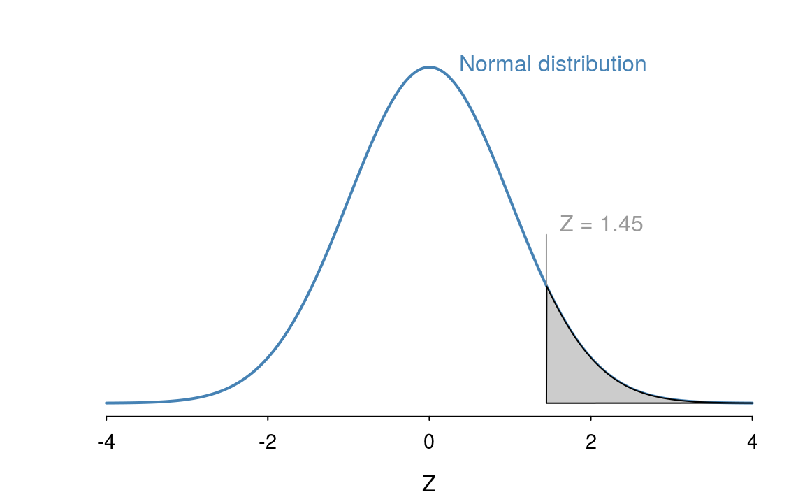
Using our example data set, if the null hypothesis is true, then \(\mu = 45\), so we have \[ Z = \frac{\bar x - \mu}{s/\sqrt{n}} = \frac{50.9 - 45}{18.2/\sqrt{20}} = 1.45 \] The obvious question is, how likely is it to have observed this value?

Since the normal distribution is symmetric, \(Z = 1.45\) is just as extreme as \(Z = −1.45\), and so the shaded region in the following diagram illustrates the \(p\)–value - the probability of observing the data we have, or anything more extreme than this, if the null hypothesis is true. In other words, the answer to our earlier question!
The closer the area of the shaded region (the \(p\)–value) is to 0, the less plausible it is that we would observe the data we have if the null hypothesis is true, that is, the more evidence we have to reject \(H_0\). So, we need to work out the area of the shaded region under the curve in the diagram above, which can be done using R
pnorm(1.45, lower.tail = FALSE) * 2
#> [1] 0.147
So the \(p\)-value is 0.15.
Earlier, we said that the smaller this \(p\)–value is, the more evidence we have to reject \(H_0\). The question now, is:
What constitutes a p–value small enough to reject H_0?
The convention (but by no means a hard–and–fast cut–off) is to reject \(H_0\) if the p–value is smaller than 5%. Thus, here we would say:
- Our p–value is greater than 5% (in fact, it’s larger than 10% – a computer can tell us that it’s exactly 14.7%)
- Thus, we do not reject \(H_0\)
- There is insufficient evidence to suggest a real deviation from the previous value
Care should be taken not be too strong in our conclusions. We can only really state that the sample does not suggest that the new design is better.
Absence of evidence is not evidence of absence
To perform the entire procedure in R, we use the t.test() function
comic = c(34, 51, 30, 79, 54, 31, 57, 62, 59, 41, 77, 55, 35, 3, 69, 46, 47, 66, 63, 59)
t.test(comic, mu = 45)
#>
#>  One Sample t-test
#>
#> data:  comic
#> t = 1, df = 20, p-value = 0.2
#> alternative hypothesis: true mean is not equal to 45
#> 95 percent confidence interval:
#>  42.4 59.4
#> sample estimates:
#> mean of x
#>      50.9
Technically this is performing a t-test which is why the associated \(p\)-value is slightly larger than our calculation. However, when the sample size is large, the t.test() function is equivalent to a z-test.
5.2.1 Example: OKCupid
The OKCupid dataset provides heights of their users. An interesting question is, how consistent are the heights given by users with the average height across the USA? First we need to extract the necessary information. R makes subsetting straightforward
## Select Males
height = cupid$height[cupid$sex == "m"]
## Remove missing values
height = height[!is.na(height)]
## Convert to cm
height = height * 2.54
mean(height)
#> [1] 179
From the CDC paper we discover the average height in the USA is 69.3 inches. We can use the \(t\)-test function in R (since the sample size is large, this is equivalent to a \(z\)-test), to obtain a \(p\)-value
t.test(height, mu = 69.3)
#>
#>  One Sample t-test
#>
#> data:  height
#> t = 3000, df = 40000, p-value <2e-16
#> alternative hypothesis: true mean is not equal to 69.3
#> 95 percent confidence interval:
#>  179 179
#> sample estimates:
#> mean of x
#>       179
Since the \(p\)-value is small, we reject \(H_0\) and conclude that the sample gives evidence that males in San Francisco are different to the rest of the USA (or just lie!).
5.2.2 Errors
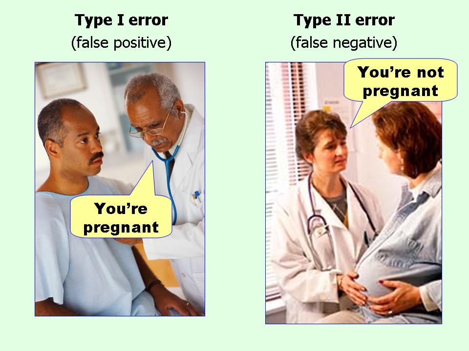
A Type I Error occurs when the null hypothesis is true but is wrongly rejected. This often referred to as a “false hit”“, or a false positive (e.g. when a diagnostic test indicates the presence of a disease, when in fact the patient does not have the disease).
The rate of a Type I Error is known as the size of the test and is usually denoted by the Greek symbol \(\alpha\), pronounced “alpha”, and usually equals the significance level of the test - that is, the p–value beyond which we have decided to reject H 0 (e.g. 5% or 0.05 in our earlier examples).
A Type II Error occurs when the null hypothesis is false, but erroneously fails to be rejected. Hence, we fail to assert what is present, and so this is often referred to as a ‘miss’. The rate of the Type II Error is usually denoted by the Greek symbol \(\beta\), pronounced “beta”, and is related to the power of a test (which equals 1 − \(\beta\)).

5.3 Two sample z-test
Suppose we want to test another improvement to our website. We think that adding a blink tag would be a good way of attracting customers. Monitoring the first twenty customers we get
21 32 46 19 29 31 37 28 50 29 34 40 26 20 48 7 39 30 40 34How do we compare the website that uses the Comic Sans font to the blinking site? We use a two sampled z-test! As with the one–sample test, we must start by setting up our hypotheses. In a two–sample z test, the null hypothesis is always that the population means for the two groups are the same \[
H_0: \mu_1 = \mu_2
\] While the alternative hypothesis is that the two pages differ, i.e. \[
H_1: \mu_1 \ne \mu_2.
\] The corresponding test statistic is \[
Z = \frac{\bar x_1 - \bar x_2}{s \sqrt{1/n_1 + 1/n_2}}.
\] This time we will jump straight into R and use the t.test() function.
blink = c(21, 32, 46, 19, 29, 31, 37, 28, 50, 29, 34, 40, 26, 20, 48, 7, 39, 30, 40, 34)
t.test(comic, blink, var.equal = TRUE)
#>
#>  Two Sample t-test
#>
#> data:  comic and blink
#> t = 4, df = 40, p-value = 3e-04
#> alternative hypothesis: true difference in means is not equal to 0
#> 95 percent confidence interval:
#>   9.37 28.43
#> sample estimates:
#> mean of x mean of y
#>      50.9      32.0
In this example, since the p-value is relatively, we can conclude that the two web-designs do appear to be different.
5.4 Confidence intervals
The idea of a confidence interval is central to statistics. When we get an answer, we don’t just want a point estimate, i.e. a single number, we want a plausible range. In fact whenever you see opinion polls in newspapers, they typically come with a margin of error of \(\pm 3\)%. It’s always amusing to see the fuss that people make when an opinion poll raises by 1% which is likely to be down to random noise.
Confidence intervals provide an alternative to hypothesis tests for assessing questions about the population mean (or population means in two sample problems), although often they are used alongside hypothesis tests. Due to lack of time, we will not cover the general theory supporting the construction of confidence intervals, although this theory is the same as that discussed in Section 4 for hypothesis tests and revolves around the Central Limit Theorem. The aim is to use the information in our sample to obtain an interval within which we might expect the true population mean to lie, with a specified level of confidence.
Recall that the sample mean \(\bar x\) is an estimate of the population mean \(\mu\). The population mean does exist; we’d like to know what it is, but usually this isn’t possible (unless we are able to take a census). The next best thing is to take a sample from the population and find \(\bar x\) - if our sample is representative of the population as a whole, we might feel confident that \(\bar x\) is a good estimator for \(\mu\), and might be close to the true value.
The problem is, if we were to take many samples from the population, and so calculate many \(\bar x\)’s, they are all likely to be different to each other. Which one would we trust the most? In reality, we don’t have the resources to take many samples, and so we’d like a way of capturing the variability of $x $ based on the information in our single sample. This is where statistical theory can help us out!
Central to the idea of margin of error, is the central limit theorem.
5.4.1 Construction
Most confidence intervals are symmetric and two–sided. Thus, to obtain a confidence interval for the population mean we:
- Find the mean in our sample, \(\bar x\)
- Subtract some amount from \(\bar x\) to obtain the lower bound of our confidence interval
- Add the same amount in (2) to our sample mean \(\bar x\) to obtain the upper bound of our confidence interval
The amount we add and subtract from \(\bar x\) is a function of the sample standard deviation \(s\) and the sample size \(n\); it also depends on just how “confident”" we want to be of capturing the population mean \(\mu\) within our interval! To be 100% confident, the lower and upper bounds would need to extend to the smallest and largest values possible for our random variable, and so it makes no sense to find such an interval; the standard is to find a 95% confidence interval.
The formula for a symmetric, two–sided 95% confidence interval for the population mean \(\mu\) is \[ \left(\bar{x}-z \times \frac{s}{\sqrt{n}}, \hspace{0.5cm} \bar{x}+z\times \frac{s}{\sqrt{n}}\right), \] often condensed to just \[ \bar{x} \pm z \times \frac{s}{\sqrt{n}}; \] where \(z\) is a critical value from the standard normal distribution. For the standard interval 95% confidence interval, the \(z\) value is 1.96, often rounded to 2. So the interval becomes \[ \bar{x} \pm \frac{2 s}{\sqrt{n}}. \] If we wanted a 90% interval, we would use \(z = 1.645\). For a 99% interval, we would use \(z = 2.576\)
5.4.2 Example: Comic Sans
Let’s return to our Comics Sans example. The average time spent on the site was \(\bar x = 50.9\) with a standard deviation of \(s = 18.2\). This gives a 95% confidence interval of \[ 50.9 \pm 1.96 \frac{18.2}{\sqrt{20}} = (42.92, 58.88). \] Alternatively, we could use R and extract the confidence interval from
t.test(comic)
#>
#>  One Sample t-test
#>
#> data:  comic
#> t = 10, df = 20, p-value = 1e-10
#> alternative hypothesis: true mean is not equal to 0
#> 95 percent confidence interval:
#>  42.4 59.4
#> sample estimates:
#> mean of x
#>      50.9
to get the interval \((42.38,59.42)\). Notice this interval is slightly wider, since it’s using the exact \(t\)-distribution.
5.5 The Central Limit Therem (CLT)
One of the reasons the normal distribution is so useful is the central limit theorem. This theorem states that if we average a large number (say 309) of variables10, then the result is approximately normally distributed.
So if we observe data, \(x_1, x_2, \ldots, x_n\), where the mean and variance of \(x_i\) are \(\mu\) and \(\sigma^2\), then \[ S_n = \frac{x_1 + x_2 + \ldots + x_n}{n} \] has a normal distribution with mean \(\mu\) and variance \(\sigma^2/n\).
The standard error of the mean is defined as the standard deviation of the sample mean, i.e. \(\sigma/\sqrt{n}\). Remember that \(\sigma\) is the population standard deviation, so we estimate the standard error using \(s/\sqrt{n}\)
5.5.1 Example: Customer waiting times

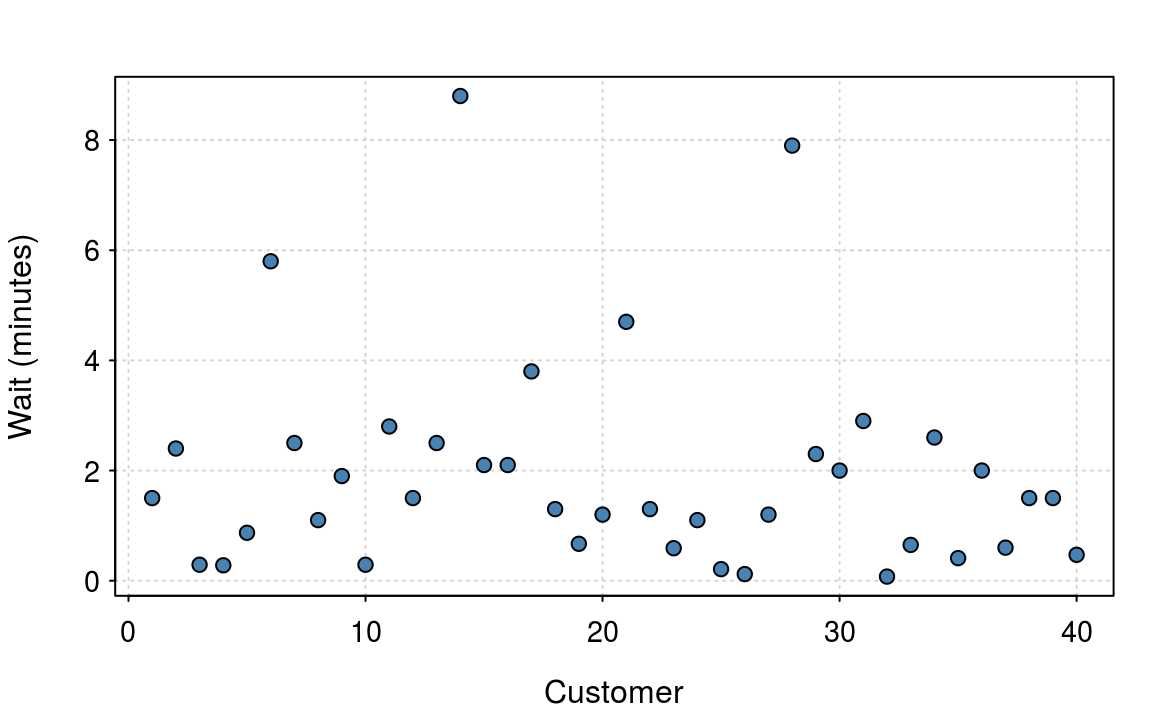
Figure 5.1: Waiting times from 40 customers. The data is skewed and is not normally distributed.
Figure 5.1 shows the waiting time (in minutes) of \(40\) customers. The figure shows that the average wait is around 1 to 2 minutes, but some unfortunate customers have a significantly longer wait. The data are clearly not normal, as waiting times must be positive and the distribution isn’t symmetric.
From chapter 2, we can quickly estimate the mean and standard deviation as 1.946 and 0.433, i.e. \(S_n = 1.946\) . The CLT allows us to take this inference one step further. Since we know that \(S_n\) is approximately normal, that implies that with probability 95%, the true mean lies between \(2.19 \pm 2 \times 2.04/20 = (1.28, 3.1).\)
Mathematically the central limit theorem only holds as \(n\) tends to infinity. However in this simple example, the underlying distribution is clearly not normal, so the confidence interval, given our finite sample, isn’t actually 95%, it’s more like 91%. Which is still not too bad.
The central limit theorem is a powerful idea. It allows to get a handle on the uncertainty whenever we estimate means. One word of warning though. If the distribution is particularly odd, then we’ll need a larger sample size for the normality approximation to be accurate.